
GPT stands for Generative Pre-trained Transformer. Generative means it produces new text. Pre-trained means it learned from massive amounts of text data before you ever interact with it — its weights are the compressed result of that learning. Transformer is the specific neural network architecture that makes modern LLMs possible.
This article explains the mechanics from scratch: how text becomes numbers, how those numbers flow through the model, and why the model's size directly determines how much memory it needs. If you prefer to learn visually: bbycroft.net/llm animates every step of the forward pass in 3D; the Transformer Explainer runs live GPT-2 inference in your browser; the 3Blue1Brown Neural Networks series covers the same concepts through illustrated video. Once you understand the concepts here, Raschka's LLM Architecture Gallery catalogs the architectural variations across more than 70 real-world models.
What is a Transformer?
The Transformer is a neural network architecture introduced in 2017 that has since become the foundation of modern AI. While this article focuses on text generation, the same architecture has been adapted for audio generation and image recognition — making it one of the most broadly applied ideas in machine learning.
For text, the operating principle is straightforward: given a sequence of input text, predict the most probable next token. That single objective — repeated over 300 billion training tokens for GPT-3 — is what produces a model capable of writing, reasoning, and answering questions. Generation is the same loop run in reverse: sample the next token, append it to the input, predict the one after that, repeat.
The core innovation that made this possible is self-attention: a mechanism that lets the model decide which parts of the input are most relevant to each token, capturing meaning and relationships even between words far apart in the sequence. Earlier architectures (recurrent neural networks) processed text one token at a time from left to right, which made it difficult to connect information across long distances. Self-attention collapses that distance — any token can directly relate to any other in a single step, regardless of how far apart they are — which is why Transformers handle long-range dependencies so much more effectively.
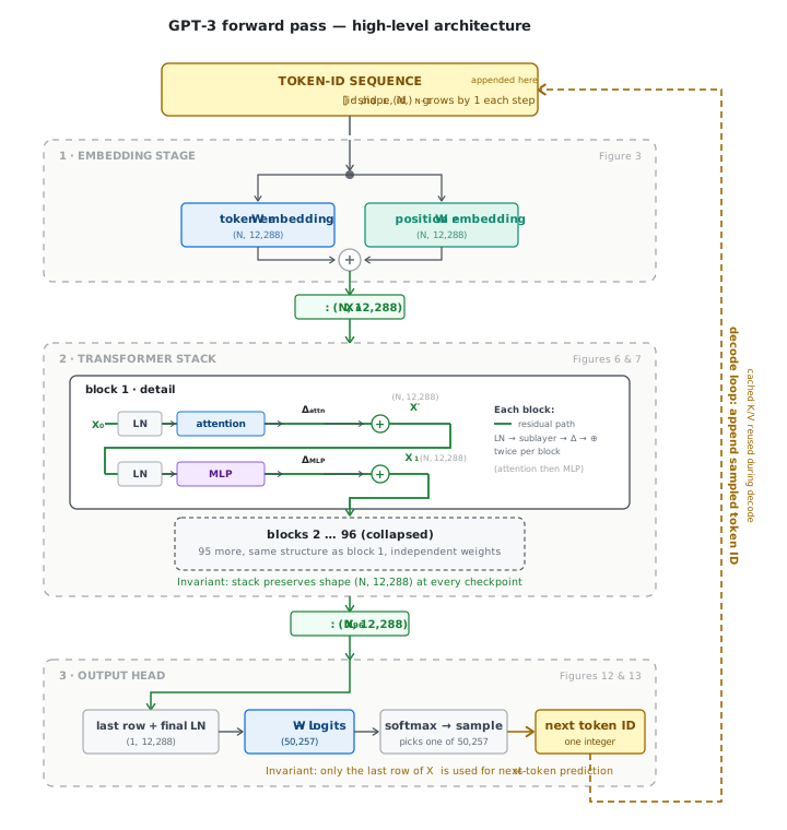
Figure 1 is the map for the rest of this article. It shows the complete path a single forward pass takes: token IDs enter at the top, flow through an embedding stage, pass through 96 identical transformer blocks, and exit through an output head that samples one next token. The feedback arc on the right is the generation loop — each sampled token is appended to the input and the process repeats.
Tokens: Text as Numbers
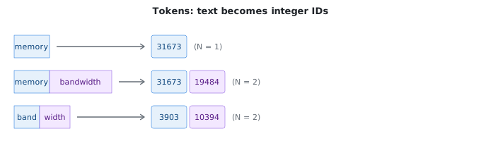
A model cannot read text. Before anything runs, your input is converted into a sequence of tokens — integer IDs from a fixed vocabulary. For text, modern vocabularies commonly range from tens of thousands to a few hundred thousand tokens; GPT-3 uses exactly 50,257. Each token represents a subword chunk: common words become a single token, rare words split into several (see Figure 2). The vocabulary is built during a separate tokenizer training phase, optimized for compression across a large text corpus. The number of tokens in a prompt determines how much computation the model needs to process it and how much memory the KV cache will consume. A 10,000-word document might be 13,000–15,000 tokens. Try the OpenAI Tokenizer to see how any text splits.
A common approach for building this vocabulary is subword tokenization, with Byte Pair Encoding (BPE) and closely related methods (SentencePiece, WordPiece) being widely used. Byte-Level BPE starts with individual bytes and repeatedly merges the most frequently co-occurring pair of units into a new token — first merging common byte pairs, then common subwords, building up to whole words for the most frequent vocabulary items. The practical benefit: subword tokenizers never produce an "unknown word" token. Any text, no matter how novel or misspelled, can be represented as a sequence of subword tokens that exist in the vocabulary. This is why models can handle code, URLs, foreign words, and typos without explicitly being trained on each one. For a deeper look at the BPE algorithm with working code, see Raschka's Implementing A BPE Tokenizer From Scratch.
Why typos still work
Typo handling is not a separate spell-checking feature. There is usually no normalization step, edit-distance search, or dictionary lookup before the model runs. The tokenizer simply converts the misspelled text into whatever subword sequence it can produce, and the transformer layers try to make useful predictions from that sequence.
For example, "artificial intelligence" and "artificial intellignece" usually become different token ID sequences, but both are still valid inputs. The typo may split into smaller or less common pieces, which gives the model a worse starting representation, but not an invalid one. Because GPT-style models are trained on noisy web text, they see misspellings, informal spelling, OCR errors, code, names, and other irregular strings in contexts that often reveal their meaning.
How the model recovers meaning from those degraded token sequences — through mechanisms described in the sections that follow — is revisited at the end of the MLP section.
Embeddings: Turning IDs into Meaning
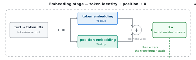
Before diving in, here is the embedding stage at a glance — each piece is explained in the sections below.
Each token ID is looked up in an embedding matrix WE — a large table of learned numbers, one row per vocabulary entry. Here is what each part of that table actually contains:
- Rows (50,257 in GPT-3) — one row per token in the vocabulary. Row 0 is the vector for token ID 0; row 31,673 is the vector for "memory"; row 50,256 is the last entry. The row index is the token ID. The lookup is literally: go to this row, return the entire row.
- Columns (12,288 in GPT-3) — the dimensions of the embedding space. Each column is one coordinate in a 12,288-dimensional space. The number 12,288 comes from the model's architecture: 96 attention heads × 128 dimensions per head (explained in the next section).
- Each cell — a single floating-point number: one coordinate of that token's position in the embedding space. Meaningless on its own. The full row of 12,288 numbers together is the representation.
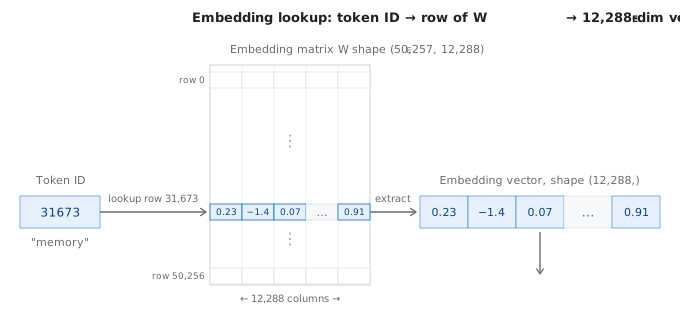
The table has 50,257 × 12,288 ≈ 617 million cells, each a floating-point number — over half a billion parameters in the embedding step alone.
The embedding matrix is a learned weight matrix — it is part of the model file, updated during training via backpropagation just like every other parameter, and stored on disk alongside the attention and MLP weights. But it sits outside the transformer blocks: it runs once at the very start (to convert token IDs into vectors) and its counterpart, the unembedding matrix WU, runs once at the very end (to convert the final vector back to token probabilities). Neither is part of any attention layer or MLP layer.
One practical note for local inference
Some engines (including llama.cpp) keep the embedding and unembedding matrices at higher precision — fp16 or fp32 — even when the rest of the model is quantized to Q4. Because these matrices are accessed as index lookups rather than matrix multiplications, quantization artifacts can be more noticeable here. So "Q4_K_M" does not necessarily mean every weight in the file is at 4-bit.
What the 12,288 dimensions represent
No single column is labeled "emotion" or "syntax" or "topic." But the geometry of the full space is absolutely structured around human-understandable concepts — sentiment, formality, syntax, semantic category, and many others. These concepts are encoded as directions: a specific combination of many columns that together point toward a region of the space associated with that concept. It is not column 47 = royalty; it is a particular direction across many columns that the model learned to associate with royalty.
A classic intuition from early static word-embedding research: the vector for “king” minus “man” plus “woman” lands near “queen.” This is a useful starting point; the geometry in full transformer models is considerably richer. Explore embedding structure visually at projector.tensorflow.org, which projects high-dimensional vectors into 3D.
Position: where in the sequence
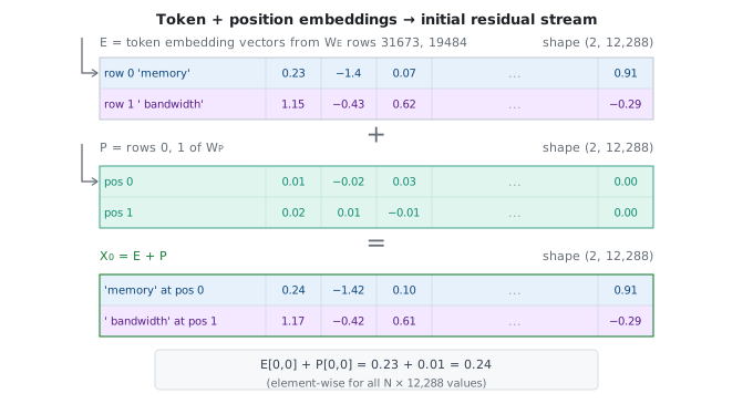
The embedding matrix WE encodes token identity but not order: the same token ID always retrieves the same row from WE, whether it appears first, tenth, or thousandth in the prompt. GPT-2 and GPT-3 handle order with a learned positional embedding table WP — a departure from the original 2017 Transformer, which used fixed sinusoidal position encodings.
GPT-3’s context window is 2,048 tokens, which means WP is fixed at exactly 2,048 rows — one learned vector for position 0, one for position 1, up to position 2,047. Because a position vector must exist in this table for a token to be processed, this row count is what determines the model's hard context limit. Each row has width 12,288 so it can be added element-wise to the corresponding token embedding row from WE. Like WE, WP is learned during pre-training by backpropagation and stored in the model file; at inference time it is just a lookup table. For GPT-3, WP has 2,048 × 12,288 ≈ 25M parameters.
For a prompt of N tokens, the model looks up N token rows and N position rows, adds them row by row, and the result is X0 with shape (N, 12,288): the initial residual stream. The residual stream is one 12,288-dimensional vector per token position, not a list of token IDs; row i is the model’s current representation of the token at position i.
Many modern LLMs instead use RoPE (Rotary Position Embedding) or similar approaches that inject positional information directly inside the attention computation. The mechanism differs, but the goal is the same: give the model a sense of sequence order while preserving each token row's 12,288-dimensional shape.
The Transformer Block
GPT models are decoder-only transformers — they generate text by attending only to previous tokens, never future ones. This is the right architecture for generation. Other architectures exist for other purposes: encoder-only transformers (like BERT) can attend in both directions simultaneously, making them better at understanding and classification tasks but unable to generate. Encoder-decoder models (like T5) combine both: an encoder reads the full input bidirectionally, a decoder generates output attending to the encoded representation. For local inference of chat and coding models, you will almost always be working with decoder-only models.
The model is a sequence of transformer blocks stacked on top of each other — 32 blocks in a typical 7B model, 96 in GPT-3. The GPT-3 paper calls these layers (n_layers = 96); this article uses “block” to distinguish the whole unit from its attention and MLP sublayers. Every block is structurally identical, but each has its own independent set of weights learned during training.
Each block contains its own attention module — in GPT-3, that means 96 attention heads per block, so a single forward pass performs 96 × 96 = 9,216 head-level attention computations in total. Heads only communicate within their own block through concatenation, WO, and the residual stream; the next block then starts with a fresh set of heads. The number of blocks and the number of heads per block are independent design choices; it is a coincidence that GPT-3 uses the same number for both.
Each GPT-3 block holds roughly 604M attention parameters + 1,208M MLP parameters; the final section breaks this down. Each block has two sublayers that operate in sequence:
- Attention — lets tokens gather information from other tokens in the sequence.
- MLP (feed-forward) — transforms each token's vector independently using learned patterns.
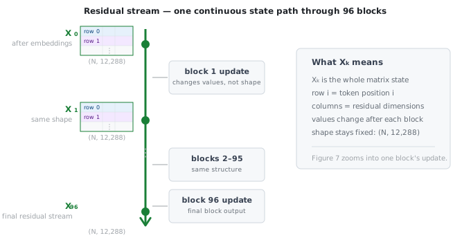
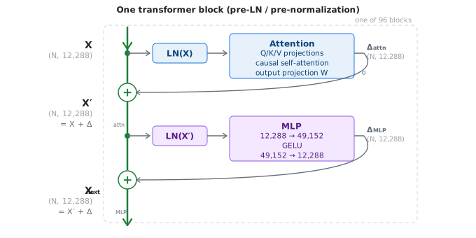
GPT-3 uses pre-normalization, inherited from GPT-2: LayerNorm is applied to the residual stream before each sublayer, and a final LayerNorm is applied after the last block before unembedding. Residual connections add each sublayer's output back into its input. This makes it easier for information to persist — each token's vector accumulates updates on top of its starting point rather than being replaced at each layer, which also helps gradients flow during training. Later layers can still attenuate or overwrite earlier features, but the path for preservation is always open. This flowing, accumulating representation is called the residual stream.
LayerNorm operates independently on each token row of the residual stream. For one token's 12,288-dimensional vector, it subtracts that row's mean, divides by that row's standard deviation, then applies learned per-dimension scale and shift parameters. This keeps the vector's scale well behaved before the attention or MLP sublayer reads it, while preserving the overall shape (N, 12,288).
Attention and QKV: How Tokens Communicate
To perform self-attention, each token's embedding is transformed into three new vectors — a query, a key, and a value. Queries compare against keys to measure how relevant each token is to every other; that relevance score then determines how much of each token's value gets passed forward. The result is a context-aware update for each token, shaped by whatever the rest of the sequence contributed.
Consider the word "mole." In "American true mole" it refers to an animal; in "biopsy of the mole" it refers to a skin lesion. The initial embedding for "mole" is identical in both cases — the same token ID, the same row in the embedding matrix. Attention is the mechanism that fixes this: it lets each token update its vector based on the other tokens around it, incorporating context into the representation.
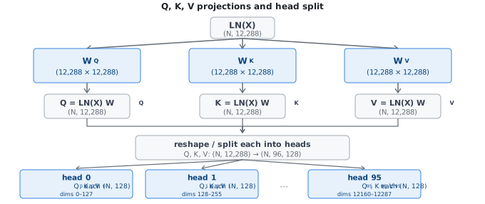
Each token simultaneously plays two roles: it asks a question about what context it needs, and it offers an answer about what it contains. The three learned projections that implement this are:
- Q (Query) — the question a token is asking. Example: "are there any adjectives before me?" Computed by multiplying the token's current vector by a learned weight matrix WQ.
- K (Key) — the label a token offers about itself. Example: "I am an adjective." Computed via WK.
- V (Value) — what a token sends when attended to. Computed via WV.
Implementation detail: diagrams often show WQ, WK, and WV as separate projections, but inference engines commonly compute them with one fused matrix multiplication and then split the result into Q, K, and V head slices. The algebra and tensor shapes are the same.
How attention computes relevance
For a given token, attention works as follows:
- Compute its Q vector by multiplying its current vector by WQ.
- Compute every other token's K vector by multiplying each of their vectors by WK.
- Take the dot product of Q with each K — positive means the key aligns with the query (relevant), near zero means unrelated, negative means they point in opposite directions. This produces a row of raw scores. In scaled dot-product attention, those scores are divided by √dhead — √128 in GPT-3 — because unscaled dot products grow with vector width and can push softmax into overly sharp, saturated distributions.
- Apply softmax to convert those scores into probabilities that sum to 1. For example, "sat" in "the cat sat down" might produce
[0.15, 0.60, 0.25, 0.00]— paying 60% attention to "cat", 25% to itself, 15% to "the", 0% to "down" (masked). Every token in the sequence does this, producing one row each. Stacked together they form the attention pattern: a context-size × context-size grid where each row sums to 1 and the strictly upper triangle is zero due to causal masking, as shown in Figure 9. Dense attention therefore has O(N²) score and weight entries for a sequence of N tokens, which is one reason long context windows are expensive. - Use each token's row of weights to blend the V vectors. "Sat" takes 60% of V("cat") + 25% of V("sat") + 15% of V("the"). The result is a change vector (Δ) — not a replacement, but an update added back into the token's residual stream, refining its representation with contextual information.
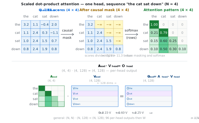
Causal masking constrains the attention pattern: each token can only attend to itself and tokens that came before it. Future tokens are masked out (their scores set to −∞ before softmax, so they receive zero probability). This is what enables the model to predict left-to-right — and it is why generation must be sequential: each new token can only see what came before it. During training, masking also enables efficiency: all token positions can be trained in parallel in a single forward pass, since each position can only see its own prefix.
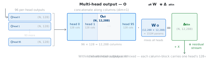
Multi-head attention runs this entire process in parallel across many independent "heads" — 12 in GPT-2 small, 96 in GPT-3. This is where the 12,288 embedding dimension connects back to what you saw in the embedding matrix:
The three quantities — embedding dimension (12,288), number of heads (96), and dimensions per head (128) — are jointly chosen and must satisfy: dmodel = nheads × dhead. Any two determine the third. The full 12,288-dimensional token vector is split into 96 equal slices, one per head, each 128 dimensions. More heads means smaller slices; fewer heads means larger slices; the total always sums back to 12,288.
What does 128 dimensions per head actually mean?
Each head is handed a 128-dimensional slice of the Q matrix and a 128-dimensional slice of the K matrix. The dot product of Q and K produces one relevance score. So 128 is the resolution of the matching: how nuanced a head's sense of "relevant" can be. With 1 dimension a head could only ask "similar or not." With 128 it can encode much finer distinctions. What each of those 128 numbers represents individually is not human-interpretable — the training process learns what Q and K should look like in 128-number space to make the attention pattern useful. 128 is a canonical choice found to work well empirically; BERT uses 64 per head, for instance.
Each head learns to specialise. One might track subject-verb agreement, another pronoun references, another long-range topic coherence. They run in parallel, their 128-dimensional outputs are concatenated back into a single 12,288-dimensional update, and the model gets 96 different "readings" of the same token at the same time.
What is stored vs what is computed
What actually lives in the model file are the weight matrices WQ, WK, WV, and WO — one set per block, learned during training, permanent. In GPT-3 each is 12,288 × (96 × 128) — input dimension × (heads × dimensions per head) — so the four attention matrices together hold 4 × 12,288 × (96 × 128) ≈ 604M parameters per block, totalling ~58B across all 96 blocks.
Q, K, and V are not model parameters — they are activations computed from the current residual-stream vectors for each forward pass. Q is used immediately to score relevance and then discarded. K and V are retained so that future tokens can attend to past ones without recomputing them. This growing collection of saved keys and values is held dynamically in memory by the inference engine as the KV cache.
Why Q is temporary but K and V persist.
Q encodes what the current token is looking for right now — it is only needed for this one step and is discarded. K and V encode what every prior token offered and sent — information that remains valid for all future decode steps. Saving them avoids recomputing the entire prompt on every new token. This is the KV cache, and it is why the memory cost of inference grows with context length, not just model size.
MLP: Where Patterns Are Stored
After attention, each token's updated vector passes independently through an MLP (multi-layer perceptron) sublayer, also called the feed-forward network (FFN) in transformer papers. Attention is about communication between tokens; MLP works on each token privately, applying learned patterns to its own representation.
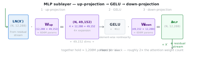
The MLP has three operations:
- Up-projection (The Keys): multiply the token vector by a large weight matrix, expanding it to a higher dimension (768 → 3,072 in GPT-2 small; 12,288 → 49,152 in GPT-3 — a standard 4× expansion ratio). With the row-vector convention used here, each column of Wup acts as a pattern detector. Research suggests that these columns act as "keys" in a key-value memory, lighting up when the token's context matches a specific learned concept.
- Nonlinearity (The Filter): apply an activation function. GPT-2/3 use GELU, a smooth alternative to ReLU; newer models often use SwiGLU. This element-wise nonlinearity acts as a filter: it squashes weak alignments to near zero, allowing only the strongly triggered pattern detectors to fire. Without this step, stacking matrix multiplications would mathematically collapse into a single linear matrix, destroying the network's depth.
- Down-projection (The Values): multiply back down to the original dimension. The rows of Wdown act as the "values" associated with the keys. When a pattern detector survives the nonlinearity, it triggers its corresponding row in Wdown — grabbing the actual stored knowledge or vocabulary update — and adds that vector back into the token's residual stream.
A concrete example of what this stores: imagine a column in Wup that acts as a key for the pattern "Michael Jordan". When those words appear in the context, that neuron activates. The corresponding row in Wdown then dumps its value — information about "basketball" — into the residual stream. Multiply this by billions of neurons across all MLP layers and you have a model that stores an enormous amount of world knowledge.
Because of this, MLPs play a major role in factual recall. Meng et al. (2022) even demonstrated that specific facts can be located in mid-layer MLP weights and surgically edited. However, saying MLPs are the only place knowledge lives is a useful approximation, not a complete picture, as attention heads and the residual stream also contribute. What is clearly true is their scale: in GPT-3 each MLP block holds Wup (12,288 × (4 × 12,288)) and Wdown ((4 × 12,288) × 12,288) — the factor of 4 is a standard expansion ratio, together ≈ 1,208M parameters per block — roughly twice the attention weight count. Across 96 blocks that is ~116B, or about two-thirds of GPT-3's 175B total.
Mixture of Experts: splitting the MLP
GPT-3 uses a single MLP per block — a dense design where every token is processed by the same MLP weights. An increasingly common alternative is Mixture of Experts (MoE), which replaces that single MLP with several expert MLPs plus a lightweight learned router. The router examines each token's representation after attention, scores it against the experts, and picks a small top-k set for that token — often 1 or 2 in early MoE models, though some modern models activate more. Each selected expert runs its own up-projection → nonlinearity → down-projection independently; their outputs are weighted by the router's confidence scores and summed back into the residual stream. In the standard transformer MoE variants discussed here, the attention mechanism is unchanged — MoE modifies the feed-forward sublayer. Despite the name, "experts" do not cleanly specialize in human-understandable domains like biology or law; research on Mixtral shows they tend to specialize at the token and syntax level, handling specific tokens in specific contexts.
The practical consequence is a split between total parameters (all experts, which determine the memory footprint because all expert weights must be available to the runtime) and active parameters (the small subset of experts used for a given token, which largely determines per-token feed-forward compute). Mixtral 8x7B has 8 expert MLPs per block and routes each token to 2, giving it 46.7B total parameters but about 12.9B active per token — memory scales like a 47B model, while feed-forward compute is closer to a 13B dense model. More recent examples include Qwen3-235B-A22B (235B total, 22B active), DeepSeek-V3 (671B total, 37B active), and Gemma 4 26B A4B (25.2B total, 3.8B active). For a thorough visual walkthrough of routing, load balancing, and the active-vs-total parameter accounting, see Grootendorst's Visual Guide; the MoE explainer from HuggingFace covers the same ground more concisely. The architecture was popularized by the Switch Transformer (2021), which showed that scaling expert count while keeping active compute roughly constant can improve quality per unit of compute.
How the model recovers from bad tokenizations
The recovery mostly happens later, through context. In “artificial intellignece”, the misspelled token starts from odd subword embeddings, but it appears beside “artificial”. Attention lets that token position gather information from surrounding tokens, and the MLP layers can contribute learned lexical and spelling-pattern associations. By later blocks, the residual-stream vector may be close enough to the intended meaning that the next-token distribution behaves normally.
This breaks down when context is weak or the typo is too far from familiar text. Random keystroke strings, rare proper nouns, technical jargon, and multilingual misspellings are harder. The model may also preserve a typo if copying the user’s exact wording or style is useful.
Superposition: How 12,288 Dimensions Hold Millions of Concepts
The embedding chapter introduced concepts as directions in a 12,288-dimensional space. With the transformer stack now in view — vectors entering from WE, then updated by attention and MLP across 96 blocks — here is how that space actually accommodates millions of concepts and what disturbs it.
Together, attention and MLP produce contextual representations: the same token can end up pointing in completely different directions depending on its surroundings. “Bank” in “river bank” and “bank” in “savings bank” start from the same row in the embedding matrix. But after the attention and MLP sublayers have updated those vectors through the transformer stack, they point in meaningfully different directions — each refined by context into a distinct representation.
An important subtlety: the model needs to represent far more concepts than it has dimensions — royalty, past tense, Python syntax, sentiment, geography, and millions more — yet it only has 12,288 dimensions. How? In high-dimensional space you can fit many more directions than you have dimensions. In 2D you can only have 2 truly perpendicular directions, but you can pack many more nearly perpendicular ones before they start overlapping significantly. At 12,288 dimensions this scales dramatically, allowing an exponentially large number of near-orthogonal directions. The model uses one direction per concept, each encoded as a specific combination of many dimensions rather than a single dedicated one. This packing strategy is called superposition.
Anthropic’s mechanistic interpretability research provides direct evidence for this structure: they found individual directions in transformer representations that correspond to remarkably clean concepts — “this is inside a quotation,” “the sentiment is positive,” “this is Python code” (Towards Monosemanticity, Bricken et al., 2023). Some features are surprisingly human-readable, but most are distributed across many dimensions and discoverable only through specialised analysis.
Quantization disturbs this because it rounds small numerical differences away. Two concepts encoded as slightly different directions may collapse to the same direction after rounding — the model can no longer distinguish them. This is one reason researchers think aggressive quantization can hurt quality disproportionately, though the precise interaction between quantization and representation quality is still an active area of research.
Unembedding: Predicting the Next Token
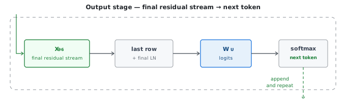
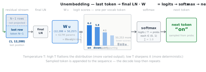
After the final block and final LayerNorm, the unembedding matrix takes the last token's vector and produces one score for every entry in the vocabulary — 50,257 scores in total for GPT-3. The last token is used because, in a causal (left-to-right) model, each token's representation encodes everything needed to predict what comes next — and the last token has attended to all previous tokens, so it carries the most complete context. These scores are called logits. (Note: Many models tie WU to WET to save parameters, though this only saves a negligible ~617M parameters in a 175B model; we show the untied accounting below).
During training and prompt prefill, every token position has a final residual-stream row and can be projected to logits for its own next-token prediction. During autoregressive generation (the token generation loop), the runtime only needs the last row: that row predicts the single next token to append.
Sampling: choosing one token from logits
The sampler converts logits into one chosen token (as visualized in Figure 13). In a typical inference runtime, the pipeline is: adjust logits with temperature and other logits processors, optionally filter candidates with top-k or top-p, apply softmax or renormalize to get probabilities over the remaining candidates, then sample one token. Libraries differ in the exact ordering of top-k/top-p and softmax, but the intent is the same: shape the candidate distribution before drawing a token.
Temperature controls how the distribution is shaped before sampling:
- Temperature = 0: implementations usually skip
softmax(logits / T)and choose the argmax token directly, giving deterministic greedy decoding. - Temperature < 1: high-scoring tokens dominate more aggressively — the model stays on-track but may be repetitive.
- Temperature = 1: raw probabilities used as-is.
- Temperature > 1: the distribution flattens — lower-probability tokens become more likely, producing more varied output, at the cost of coherence at high values.
Temperature is a probability-shaping parameter, not a creativity or reasoning dial: it changes how aggressively the sampler favors high-scoring tokens after the model has already computed its logits.
Top-k sampling further limits the candidate pool to the k highest-probability tokens; top-p (nucleus) sampling keeps only the smallest set of tokens whose probabilities sum to at least p.
The Generation Loop: Prefill Then Decode
A complete inference run has two distinct phases with fundamentally different performance characteristics:
Prefill processes the entire input — system prompt, conversation history, tool schemas, user message — in one forward pass. All tokens flow through the transformer in parallel. This exploits the GPU's ability to perform massive matrix multiplications across the full sequence simultaneously. Prefill is compute-bound: the speed is limited by how fast the GPU can perform arithmetic. The result is the first generated token and a fully populated KV cache for every input token.
Decode generates output one token at a time in an autoregressive loop — each generated token is appended to the input and becomes context for the next step. Each step processes only the newest token: compute its Q, K, and V; append the new K and V to the cache; run attention against the full cache; run MLP; project to logits; sample the next token. Then repeat. Because each step processes just one token instead of the full sequence, the GPU performs far less arithmetic but must still read the entire model weight set and the full KV cache from memory. Decode is memory-bandwidth-bound: the GPU spends most of its time waiting for data to arrive from memory, not computing.
Throughout the rest of this section, t refers to the current decode position. Before step t begins, the cache holds K and V rows for positions 0 through t−1. The step computes Qt, Kt, and Vt for the new token, appends Kt and Vt to the cache, then uses Qt to attend over all t+1 positions — the current token attends to itself as well as every earlier token.
Table 1. Comparing Prefill and Decode. Prefill runs once per request and is compute-bound; Decode runs iteratively per token and is memory-bandwidth-bound.
| Aspect | Prefill | Decode |
|---|---|---|
| How often | Once per request | Once per generated token |
| Input token IDs | Full prompt, shape (N,) | Newest token only, shape (1,) |
| Residual stream | (N, 12,288) | (1, 12,288) |
| Q/K/V computed for | All prompt tokens | Newest token only |
| Attention per head | (N, N) attention pattern | (1, t+1) attention row over positions 0 through t |
| KV cache | Created and populated for all prompt tokens | Read, then extended by one K row and one V row |
| Unembedding | Only the last row is needed for generation | The single row is projected to logits |
| Main bottleneck | Compute-heavy matrix work | Memory bandwidth: weights and growing KV cache |
Same weights, different leading dimension. Prefill batches the whole prompt through the model once; decode repeatedly calls the same model one token at a time, reusing cached K and V from earlier tokens. That shape change is why prefill is good at using GPU arithmetic throughput, while decode is dominated by reading weights and the growing KV cache from memory.
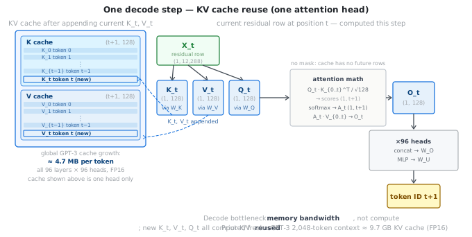
This is why memory bandwidth (GB/s) predicts local inference speed — not GPU compute power (TFLOPS), not clock speed.
Every new decode step reads the cached K and V instead of recomputing them from scratch. For GPT-3 at FP16, each token adds 2 (K and V) × 96 layers × 96 heads × 128 dimensions × 2 bytes ≈ 4.7 MB of KV cache. A full 2,048-token context is about 9.7 GB in decimal units, or about 9.0 GiB, separate from the roughly 350 GB needed for FP16 weights. Modern long-context systems can be much cheaper because GQA/MQA use fewer K/V heads, runtimes can manage the cache in pages or blocks, and some also quantize the KV cache.
The size of the cache depends on the model’s architecture. A model with fewer KV heads (GQA) has a dramatically smaller cache than one with full multi-head attention — one of the practical reasons modern models favour GQA.
The attention description above covers standard dense multi-head attention (MHA). To avoid the O(N²) memory bottleneck, modern implementations compute this exact attention using FlashAttention, which vastly speeds up the compute-bound prefill phase without ever materializing the full attention matrix in GPU memory. Real models also vary significantly in their attention patterns: GPT-3 itself alternated dense and locally banded sparse attention layers; Grouped-Query Attention (GQA) shares K/V heads across query groups to cut memory; Multi-head Latent Attention (MLA) compresses K/V into a smaller latent vector; Sliding Window Attention (SWA) limits each token to attending only nearby tokens for long-context efficiency. Raschka’s A Visual Guide to Attention Variants in Modern LLMs covers all of these with diagrams.
One consequence of the autoregressive loop: the model can only work within a fixed context window — the maximum number of tokens it can process at once. This is a hard architectural limit set during training (GPT-3 used 2,048 tokens; modern models typically support 32K to 262K). Everything the model knows about your request must fit inside this window: system prompt, conversation history, tool schemas, documents, and the response being generated. Tokens that fall outside the window are simply invisible to the model.
Speculative decoding: breaking the one-token-at-a-time barrier
Standard decode is strictly sequential — causal masking means each token must exist before the next can be computed. But the hardware is underutilized during decode: the GPU reads the full weight set and KV cache from memory yet performs very little arithmetic on that single token. Speculative decoding exploits this idle compute by having a fast, cheap source propose several draft tokens at once, then verifying all of them in a single parallel forward pass through the full model — similar in cost to prefill, where batch processing is efficient. Tokens the full model agrees with are accepted; the first disagreement triggers re-sampling at that point, and the draft cycle restarts. Because verification uses rejection sampling, the output distribution is mathematically identical to standard decoding — there is no quality loss.
The two main approaches are draft-model speculation, where a separate smaller model (typically 0.5B–3B) proposes tokens (llama.cpp supports this via `--model-draft`), and Multi-Token Prediction (MTP), where the model is trained with auxiliary prediction heads that draft from the target's own representations, without a separate standalone model — Google’s Gemma 4 ships with MTP heads, reporting up to 3× speedup, and Ollama merged native MTP support for Gemma 4 on Mac. A third family, EAGLE, attaches a lightweight trained prediction head to the target model’s internal representations; EAGLE-3 checkpoints are available on HuggingFace for Llama 3.3 70B, Qwen3, and others, and are supported by vLLM and SGLang.
Speculative decoding is becoming a standard inference optimization — it targets the decode bandwidth bottleneck directly by producing multiple accepted tokens per full-model memory read.
Training vs. inference.
The forward pass described above is inference — generating output from a fixed model. During pre-training, the same forward pass runs on enormous amounts of text with a simple objective: predict the next token. The error between the predicted probability and the actual next token is used to adjust every weight in the model through backpropagation. For GPT-3, this process covered 300 billion token positions. After pre-training, a base model exists that can predict text but does not yet follow instructions. A second training phase — instruction fine-tuning, often combined with reinforcement learning from human feedback (RLHF) — teaches the model to be helpful, follow directions, and decline harmful requests. The result is what you interact with as a chat or coding assistant.
Emergent abilities.
A striking property of large-scale pre-training is that models develop capabilities they were never explicitly trained for. A model trained only on next-token prediction can perform translation, summarization, arithmetic, code generation, and logical reasoning — not because these tasks were in the training objective, but because they are implicit in the patterns of a large enough text corpus. These are called emergent abilities: they appear at sufficient scale and are largely unpredictable in advance. Few-shot learning (performing a task from just a few examples in the prompt) and zero-shot generalization (performing a task with no examples at all) are the most practically useful manifestations of this.
Why Model Size Equals Memory Requirement
Every learned parameter described above is a floating-point number that must live in memory while the model runs. For GPT-3, the full tally:
- WE (embedding matrix): 50,257 × 12,288 = ~617M
- WP (learned position embeddings): 2,048 × 12,288 = ~25M
- Attention weights (WQ, WK, WV, WO): 4 × 12,288 × (96 × 128) × 96 blocks = ~58B
- MLP weights (Wup, Wdown): 2 × 12,288 × (4 × 12,288) × 96 blocks = ~116B
- WU (unembedding matrix, if untied): 12,288 × 50,257 = ~617M
- Biases and LayerNorm parameters: ~15M — negligible at this scale
- Total with untied WU: ~175.2B
- Total with tied WU = WET: ~174.6B
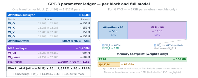
Published model sizes are rounded, so both accounting conventions are compatible with the advertised 175B-parameter scale.
The KV cache is a separate runtime allocation on top of these weights — it is not part of the model file but competes for the same memory pool during inference.
At full 16-bit precision (BF16 or FP16), each parameter occupies 2 bytes. A model with B billion parameters requires approximately 2B bytes — 2 GB per billion parameters — just for the weights. A 70B model at FP16 needs ~140 GB before the KV cache is even considered.
Quantization reduces this by storing weights at lower bit widths. A 4-bit quantized model (Q4_K_M) uses roughly 0.5 bytes per parameter, cutting the 70B footprint to ~40 GB. The tradeoff is precision loss: quantized values are approximations of the originals. The relationship between quantization aggressiveness and quality degradation is not linear — and because of superposition, the impact depends heavily on which weights are compressed and how the model uses them.
By this point you’ve traced the full forward pass: tokens become vectors via WE and WP; the residual stream flows through 96 transformer blocks that update it via attention (token-to-token communication) and MLP (per-token pattern application); the final residual-stream row is projected through WU to logits and sampled. Generation is the same pass repeated once per token, with K and V cached so prior tokens never need to be re-encoded.